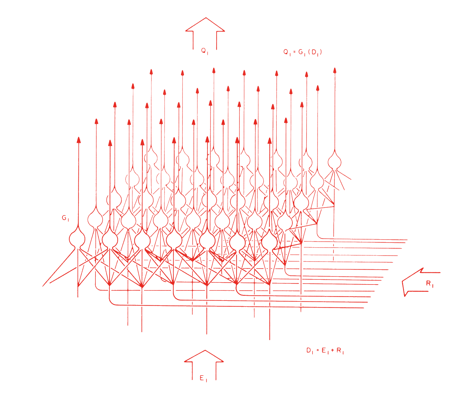
Byte Magazine, August 1979
Cleanliness is Next to Godliness
Developmental flow
How does learning produce understandable structure? What a neural network learns can change what it learns next. Each acquisition modifies circuitry that later training can build on, making certain features easier or harder to acquire. Those dependencies can give otherwise disparate responses a coherent developmental history.
In Neural Networks Are Already Clean, Nick Cammarata tracks one such developmental history in a retrained InceptionV1 model.1 A neuron initially responds most strongly to yellow-flower images that may or may not contain dogs. As training continues, the neuron responds strongly to green objects, dogs pictured without flowers, and eventually broccoli.
Cammarata calls this “recursive generalization.” As a neuron learns to respond to related inputs, the features it detects can provide a basis for learning others. He interprets neurons through the distinctions they draw for downstream computation, even when their responses cross familiar categories.1 Cleanliness, in his account, means that varied responses have an intelligible computational role and developmental history.
Features are the learned patterns or distinctions that neural mechanisms implement. I use path formation to describe how training reshapes circuitry and changes what becomes easier to learn next. An acquired feature can change how later learning signals reach and modify that circuitry, making another feature easier to acquire. The flower timeline motivates this explanation, while the specific causal connections remain hypothetical.
One path leads to another
Explaining the flower neuron’s changing responses requires examining the circuitry that determines its activation and uses its output. Cammarata’s circuit-ecology hypothesis proposes that established pathways capture learning signals ahead of competitors built from scratch. In his account, improvements through established pathways reduce error and can weaken competing pathways’ learning signals for the same task.1
The path formation account developed here starts with a flower-responsive mechanism that also responds weakly to vegetation, animals, or shared textures. When green-object examples activate it, the training loss can produce gradients through its downstream connections. Compatible gradients could strengthen its green response, providing an input for a later broccoli detector. In the illustrated case, reusing and modifying that circuitry requires fewer training steps than developing the signal independently.
Learning pressure describes how training signals favor changes in existing circuitry. Reinforcement and suppression refer to a specified contribution or response, and pressure magnitude is distinct from the change it produces. Lowered resistance means fewer optimization steps or examples under comparable conditions, an advantage that strong activation or gradient support alone does not establish. Where that advantage exists, earlier distinctions help explain how a new feature develops.
Two paths, one distinction
Cammarata compares InceptionV1 and ConvNeXt neurons that initially respond to rapeseed fields but develop different sets of strongest responses.1 These shifts need not erase responsiveness to earlier categories. Architecture and learning history both differ, so the comparison motivates a question about later learning costs without isolating their cause.
Consider two networks whose internal representations preserve the same flower distinction over a specified set of flower and nonflower inputs. Both group the inputs alike for this distinction and make it available to downstream computation. The networks share the same layers and possible connections, but different learned weights implement that distinction through different pathways. Both receive the same subsequent examples under the same optimization procedure.
Preserving the same distinction does not make these pathways equally easy to modify. In World A, learning the broccoli feature through the flower mechanism could reduce activation on flower inputs and compromise computations that depend on that signal. World B illustrates a separate route that could preserve both roles but require more training. The distinction describes which inputs the representations separate, while the processes implementing it shape how that separation can be reused or changed.
Learning pressure changes roles and responses
Training can change both how much a mechanism contributes to later computations and what it detects. Those changes determine the contribution weights and trait changes in the Price equation. They are two effects of the same learning pressure and need not point in the same direction. Price’s equation separates their contributions to a change in a measured trait, such as responsiveness to dogs without flowers.2
To apply it, fix a population of earlier flower-related mechanisms, a set of tasks, and a rule attributing later uses to those mechanisms. Divide credit for each later use among its contributing mechanisms. A mechanism’s total credit gives its weight $w$, while $z$ measures its response on fixed test images and $\Delta z$ measures response change in its later uses.3
\Delta\bar z
=
\underbrace{\frac{\operatorname{Cov}(w,z)}{\bar w}}_{\text{selection}}
+
\underbrace{\frac{\mathbb E[w\Delta z]}{\bar w}}_{\text{variation}}.
The equation is a mathematical decomposition of change and does not itself establish causality.
The selection term is positive when mechanisms already responsive to dogs receive greater relative weight. Its sign gives the direction of this contribution, and its magnitude gives the shift in the mean response due to weighting. More total contribution alone does not imply a shift toward dog responsiveness. What matters is how contribution is distributed across the earlier traits.
Variation, the standard transmission term, captures response changes within inherited mechanisms and their later uses. It weights those changes by their contributions. Selection toward dog responsiveness could be offset by variation away from it, leaving the average unchanged despite substantial development.
The bands depict proposed training pressure, while the Price terms account for its stipulated consequences under the attribution rule. Pressure magnitude alone determines neither term, since the outcome also depends on the circuitry and its response to training. If each neuron instead has one equally weighted continuation across checkpoints, then $w_i=1$ and selection is zero, even when gradients compete. All measured response change then enters variation.
In the hypothetical training interval below, pressure favors additional contributions from dog-responsive mechanisms and dog responsiveness in a previously nonresponsive inherited use. Reweighting the earlier traits accounts for a rise from 50% to 75%, while acquisition of the trait accounts for the remaining rise to 100%. Selection and variation reinforce each other here, each contributing 25 percentage points.
How learning builds understandable structure
A mechanism’s current response does not fully describe its developmental role. Mechanisms that respond alike can differ in how training changes them and what later computations can build on them. Learning pressure can redistribute their contributions before an activation summary reveals the difference. The changed circuitry then channels later training signals, potentially making different extensions easier to learn.
Price’s equation separates changes in contribution from changes in measured traits, but neither a current average nor its immediate change necessarily determines what follows. Under specified selection dynamics, populations matching both can later diverge because their internal composition differs. Applied to neural learning, this suggests that an apparently stable feature can conceal a changing developmental trajectory, a possibility the flower timeline alone cannot establish.
A shared pathway could contribute more to broccoli detection while becoming less responsive to flower inputs. Other pathways may lose relative influence while remaining available, making some later acquisitions harder without making them impossible. Present learning advantages therefore need not preserve every future opportunity, and retaining the flower role may require new circuitry even as broccoli becomes easier to learn.
Learning can produce understandable structure because each acquisition builds on distinctions already available and reshapes the opportunities that follow. In this account of Cammarata’s recursive generalization, disparate responses become intelligible through the dependencies connecting their development. A network’s apparent cleanliness can reflect that accumulated organization, including changes in both what its features detect and what later computations build on them. Learning builds the machinery of its own future learning.
Cammarata, N. (2026). Neural Networks Are Already Clean. Goodfire.
Price, G. R. (1970). Selection and Covariance. Nature, 227, 520–521.
Price, G. R. (1972). Extension of covariance selection mathematics. Annals of Human Genetics, 35, 485–490.
Frank, S. A. (1997). The Price Equation, Fisher’s Fundamental Theorem, Kin Selection, and Causal Analysis. Evolution, 51(6), 1712–1729.
Take equally weighted baseline mechanisms with fixed assay responses $z_i$. Assign each included later use one unit of credit, divided among its registered ancestors, and exclude unassigned uses from this population. Let $w_i\geq0$ be an ancestor’s total credit and $\Delta z_i$ its credit-weighted descendant mean response minus $z_i$, set to zero when $w_i=0$. Expectations and covariance use the baseline population, $\bar w=\mathbb E[w]>0$, and $\Delta\bar z$ is the later attributed-use mean minus the baseline mean.45